 Fellow Daoist
A Quick Tour of XGBoost
An applied practitioner's tour of Gradient Boosted Decision Trees and XGBoost - where it came from, how it actually works under the hood, and understanding why it works so well on tabular data
What is This for?
In the world of applied ML, a good chunk of the tasks fall into the domain of tabular data thanks to how handy the tabular form is. It shows up everywhere, from banking, to marketing, healthcare, and retail, just to name a few - it's simply a tabular world out there!
Therefore, this is a well-studied domain with a plethora of known approaches to tackle it at scale, and one of the most successful ones with widespread adoption and great baseline performance, is the Gradient Boosted Decision Trees (GBDT) class of methods, of which XGBoost is one of its most popular instantiations. A short, non-exhaustive listicle of where it shows up in practice:
- Kaggle dominance - in winning tabular solutions since 2015, from the ASHRAE Great Energy Predictor III to the TabArena living benchmark
- The Higgs boson challenge, high-energy physics
- Credit scoring and loan default forecasting
- Medicare fraud detection
- The default tabular baseline in benchmarks - Grinsztajn et al., Shwartz-Ziv & Armon, McElfresh et al.
- Still ahead of tabular foundation models past ∼104 rows - see A Closer Look at TabPFN v2
- Ahead of tuned deep nets and deep sequence models at scale
The question then arises, what makes them such effective algorithms and how do they work under the hood? [1]Per my own experience, the concept and theory of Decision Trees are widely known amongst practitioners as it's widely taught in schools. GBDT however, much less so! This short essay sets out to answer this exact question from an applied perspective instead of a dense rigorous treatment, as there are already many existing texts on that - The Elements of Statistical Learning and Boosting: Foundations and Algorithms - and I am personally much more interested in knowing what makes it tick and the reason behind its unreasonable effectiveness out-of-the-box. The end goal is to provide a sufficient technical exposition in an intuitive yet grounded way, and then leverage that understanding to answer the aforementioned question, which hopefully will help my fellow practitioners make better decisions with these tools in their day-to-day work.
A Little Historical and Ontological Detour
The idea of iterative refinement by combining a collection of weak learners to yield a stronger learner is a pretty intuitive one in retrospect, and this is exactly how GBDT works - it combines many Decision Trees into a "super-tree" in a specific way such that the super-tree is more powerful than its constituents.
One of its roots can be traced back to Kearns and Valiant (1989; J. ACM 1994) in PAC learning [2]Which has one of the funniest names in my opinion - Probably Approximately Correct Learning, ha! when they tussle with the question of whether it's possible to create a strong learner (model) with arbitrarily low error by combining only weak learners, that individually, are only marginally better than random!
Turns out - yes you can, and this gave birth to the ensemble class of methods we all know and love today. I'll skip over straight to the landmark result - for brevity - of AdaBoost (Freund and Schapire, 1997), and this miraculous algorithm, although simple in concept, was shown to be able to drive training error to 0 exponentially-fast, and more interestingly its test time error continues to improve even after the training error has hit 0! In short and with great deal of simplification, AdaBoost works by maintaining a distribution over its training samples. As the successive weak learners get trained and "combined" into the wider structure of the super-learner, the training samples used to fit each successive weak learner are reweighted (up or down weighted) so as to prioritize - give a boost (!) - the samples where it's making mistakes. The idea, is to learn with more emphasis on the "hard" samples to get them right next time; for output, it uses a simple weighted voting mechanism amongst weak learners (each weighted by a scalar, αm) to decide on what the final value of the super structure would be. Pretty straightforward!
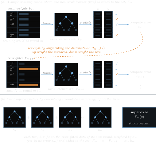
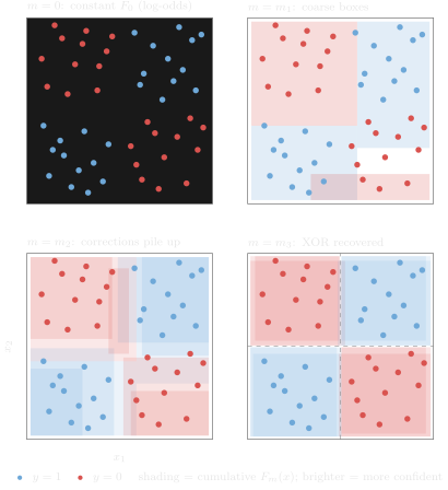
Then Friedman (2001) took it a step further, and suggested the idea of fitting each new weak learner to the negative gradient of the loss with respect to the pseudo-residuals, for any differentiable loss, to drive the iterative adaptation process - hence, Gradient Boosting! This essentially recast the solution from a reweighting one, to a numerical optimization task. Written out, the ensemble after m rounds is just the previous ensemble plus one more tree, and that tree is itself just a piecewise-constant function over the regions its splits carve out:
Fm(x)hm(x)=Fm−1(x)+ηhm(x),=j=1∑Tmwmj1{x∈Rmj}.where
| Symbol | Meaning |
|---|---|
| x | the feature vector of a single sample |
| m | the index of the current boosting round, m=1,…,M |
| Fm | the ensemble ("super-tree") after m rounds |
| Fm−1 | the cumulative output from the learner sets of all prior rounds [0,…,m−1] |
| hm | this round's weak learner (a single tree) |
| η | the learning rate (or shrinkage) |
| Tm | the total number of leaves in round m's tree |
| Rmj | the j-th leaf region - an axis-aligned box carved into the feature space by the nodes and leaves of this round's tree |
| wmj | the leaf weight, a constant value the tree outputs on Rmj |
| 1{⋅} | the indicator function: 1 when x falls in that region, 0 otherwise |
Note that for a single tree at round m, the regions Rm1,…,RmTm are disjoint and cover the whole feature space, so for any given sample on the manifold, x will only fall into a single region and hence be associated with only a single leaf weight as per the tree equation above. Across trees however, the regions Rmj from different rounds m can overlap and it is this cumulative iterated segmentation that produces the final margin. Then simply apply a threshold, and voila(!) out pops the class.
XGBoost Proper
Now we have a GBM (Friedman, 2001) that is nice to deal with in the form of a familiar optimization problem, where we can "intelligently" learn an "optimal" ensemble (boosting) model by stacking weak learners in an end-to-end manner - and indeed it's pretty effective! However, it still has some clunky bits and gaps, and it took Chen and Guestrin in 2016 to finally bridge those gaps with the XGBoost that we know and love today. There are a lot of engineering tricks and clever reformulation that made XGBoost so much better than GBM, and so well adapted to the real-world, large-scale workloads we see in practice, but in the interest of time, I'll focus only on the core, and most consequential bits, providing a necessary and sufficient exposition to the question of "how does it work?"
Reformulation as a Regularized Objective
Friedman's GBM already had shrinkage, subsampling and tree-size limits, and Newton-step boosting existed (LogitBoost). What XGBoost did was fold the explicit penalties γT+21λ∥w∥2 into the second-order objective so that leaf weights and split gains come in as a single closed-form parcel, and most importantly, did a lot of polishing to engineer the whole thing to scale. By reformulating the learning task as a regularized objective, it in one shot naturally deals with regularization and adverse spurious sample selection in a single pass, instead of a cascade of steps, enabling stabler learning even with tricky datasets.
The objective function
For a regularized objective at round m, and with the previous m−1 trees frozen (so their Ω terms are constant and dropped), we have
L(m)=i=1∑nℓ(yi,y^i(m−1)+hm(xi))+Ω(hm)where i is the sample index, and y^i(m−1) is the output from Fm−1. Also, for simplicity, we're just gonna deal with a binary classification task, therefore the loss is simply the Binary Cross-Entropy.
ℓ(yi,y^i)=−yiy^i+ln(1+ey^i).The regularizer
Ω(hm)=γT+21λj=1∑Twj2+αj=1∑T∣wj∣Ω(hm) is the regularization term for learner hm (writing T and dropping the subscript for brevity), and can be broken down as follows:
- Leaf-count penalty γT (
gamma) - penalizes the number of leaves. This is a simple additive cost per leaf on the number of total leaves, T, so as to prevent over-splitting of nodes and to make sure each split is done only with sufficient loss reduction in return. - L2 shrinkage 21λ∑j=1Twj2 (
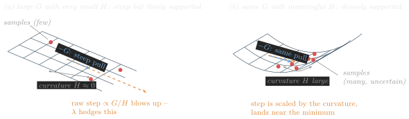
lambda) - penalizes the magnitude of the assigned leaf value. It effectively tries to push each wj toward 0, so more emphasis is placed on meaningful samples only. This is most aggressive where Hj (Hessian or curvature) is small (lots of spurious samples). - L1 sparsity α∑j=1T∣wj∣ (
alpha) - also penalizes magnitude and additionally encourages sparsity: it can drive a wj exactly to 0.
As a whole, the above should be a familiar expression for those with some optimization background: this is just a regularized objective. As an aside, the 21 on the L2 term is just a mathematical nicety - it cancels on differentiation and keeps the later expression for w∗ tidy for those picky statisticians. Also, everything below assumes α=0.
From First Order to Second Order Estimation
XGBoost also uses 2nd order optimization rather than 1st order so as to account for not only the gradient, G, but also the curvature of the loss landscape, H (the Hessian, in fancy-speak). This is super helpful throughout the learning process, such that it enables the learners to not only determine the direction of steepest descent, but also one that's nicely conditioned. To see why it matters, let's define the gradient and curvature terms first:
Gradient and Hessian
Both are derivatives of the (binary cross entropy) loss with respect to the model's output, evaluated at the current margin, y^i(m−1):
Gi=∂y^∂ℓ(yi,y^)y^=y^i(m−1)=σ(y^i(m−1))−yi=pi−yi, Hi=∂y^2∂2ℓ(yi,y^)y^=y^i(m−1)=pi(1−pi).where
- Gi∈(−1,1) - a signed error. Gi<0 means the margin must increase and vice versa.
- Hi∈(0,0.25] - the local curvature, maximal at pi=0.5 (most uncertain). This effectively acts as the support mass of a leaf - large where the model is least confident, and it dampens the step w∗ there rather than amplify it, and vice versa.
Basically, the gradient provides the signal of "where to go" with respect to the current loss landscape, and the curvature then characterizes where the most interesting regions are, given what the model currently knows (and doesn't know).
Optimal leaf weight
Next, we see where G and H are directly applied - specifically in computing the optimal leaf weight wj∗ of each leaf j for a particular tree, hm. Very conveniently, each leaf j contributes Gjwj+21(Hj+λ)wj2 to the objective (we'll derive this in the next section) where λ>0 is a regularizing term. Therefore, by setting the derivative to zero, the optimal weight wj∗ admits a closed form solution:
∂wj∂[Gjwj+21(Hj+λ)wj2]=Gj+(Hj+λ)wj=0 wj∗=−Hj+λGj=−∑i∈Ijpi(1−pi)+λ∑i∈Ij(pi−yi)Obviously, the second derivative is Hj+λ>0, so this is a minimum. Note that λ serves to dampen the weights of leaves built on little Hessian mass (e.g. nothing much to learn). So now, we have a way to condition the learning on the "informativeness" of certain samples at a given round with H, and control for how much emphasis should be placed on it with λ.
Very Smart Plumbing
Chen and Guestrin really went the extra mile to make sure that XGBoost is practically useful. One good example, is how it puts into practice what we've just covered, to efficiently evaluate the gradient, G and curvature H, in its objective function!
Second-order surrogate
As nice as the regularized objective is, it unfortunately has no closed-form minimizer over tree structures and weights, and hence we need some way to go around this; the common toolkit to solve such functions is iterative and slow; this would be a tough sell for learning with large-scale datasets, which are so prevalent in the wild (e.g. transactions at Stripe each hour, number of Uber bookings per day). Therefore, XGBoost introduced a surrogate as a bypass, by simply taking the second-order Taylor expansion of the function, which can be easily evaluated directly and is sufficiently representative at local-scale (which our Trees are operating at). Taylor-expand the objective to second order around y^i(m−1) and drop the constant ℓ(yi,y^i(m−1)), and that yields:
L~(m)=i=1∑n[Gihm(xi)+21Hihm2(xi)]+γT+21λj=1∑Twj2Every sample in leaf j receives the same output wj, so regroup the sum w.r.t. each leaf, then
L~(m)=j=1∑T(i∈Ij∑Gi)wj+21(i∈Ij∑Hi+λ)wj2+γTNow, let's make this a bit nicer to write by defining the leaf aggregates
Gj=i∈Ij∑Gi,Hj=i∈Ij∑Hiwhere i are samples at node Ij, and therefore
L~(m)=j=1∑T[Gjwj+21(Hj+λ)wj2]+γT.Take a moment and notice that the above is T one-dimensional quadratics in wj. The sample index i has vanished and a leaf is now just the pair (Gj,Hj). This makes downstream terms much easier to organize and compute exactly with the gradient, Hessian and optimal-leaf-weight expressions we've already derived!
Structure score
We can go further, and use the same idea to also determine how a tree should split at each node with what we have already derived. Substitute wj∗ back, and summing over all leaves we can see that the tree scores exactly
L~∗(q)=−21j=1∑THj+λGj2+γTThis is the quality of a tree structure q (tree spawned at round m) - of course, lower is better. It plays the role that impurity / Gini plays in a classification tree, but derived from the actual loss directly. And from the above, we can also define the per-node score, S(I) as
S(I)=HI+λGI2.What we have done so far, is to show that at the heart of XGBoost, the optimal value of a leaf and the quality of a learned tree (weak-learner) are explicitly parameterized as functions of the first, G and second order, H statistics for any twice-differentiable loss function - very nice! Next, we need a way to compare before vs after a split to quantify whether a split is worth it or not. We do so by introducing a new function called the Gain as such
Gain=unsplitL~∗(before)−splitL~∗(after)Consider splitting node I into IL (left) and IR (right), such that I=IL⊔IR (disjoint), and because GI and HI are simply sums of Gi and Hi, therefore
GL+GR=GIHL+HR=HIThis makes it trivial to recover either side once we have accumulated G and H for one side. Also, as one node splits into two, T increases by exactly 1, thereby accruing an additional penalty of 1×γ. By substituting the structure score into the Gain equation and making use of the sum decomposition above, we arrive at the full Gain equation as follows
Gain=21left childHL+λGL2+right childHR+λGR2−parent, unsplitHL+HR+λ(GL+GR)2−γwhere
- Left child score HL+λGL2 - how much loss the left branch can reduce
- Right child score HR+λGR2 - how much loss the right branch can reduce
- Parent score HL+HR+λ(GL+GR)2 - how much loss the parent node can already reduce by itself without splitting
- γ - the additional leaf-penalty we've incurred by splitting one-to-two
XGBoost's simple yet effective strategy is to simply greedily pick the action with largest Gain! Notice the Gain is zero only when the two children want the same weight, GL/(HL+λ)≈GR/(HR+λ), in which case one shared weight already captures it and the split is pointless. Opposite-sign gradients, where the L/R branches want to move the margin in different directions are the clearest case of disagreement, meaning there's something worth splitting on here, and same-sign gradients with different magnitudes or curvature also produce positive Gain. In order for a split proposal to be accepted, by default, it needs to have a positive Gain value, such that
maxGain>0⟺21[HL+λGL2+HR+λGR2−HI+λGI2]>γ,so γ is literally the minimum loss reduction a split must induce. The routing rule is then simply: for samples where xk∗<v∗ go left, else right, subjected to two additional structural constraints:
min(HL,HR)≥min_child_weight,depth≤max_depth.min_child_weight is a cutoff on Hessian mass so that only gradient induced by sufficiently meaningful or salient samples, not sample count, will be considered in the Gain equation; there's not much meaning creating more splits on already well-classified data points. For example, a child of 50 confidently-classified samples (Hi≈0) will fail the cutoff, while a child of 5 uncertain ones passes and can have a positive Gain since there's something worth learning here still. max_depth is pretty self-explanatory, it's just the maximal depth limit of the tree, hm that we explicitly define and enforce; this is to prevent overfitting since a tree of depth D, can model interactions up to order of D.
In effect, all these mechanics replace tedious per-leaf optimization with simple closed form evaluation with just 2 computed scalars (λ and γ are fixed) that we can precompute in a batch ahead of time, and thus when it comes time to determine the split at a given node j, we can just do a series of fetch-and-sum! Not only that, with some clever arrangements, we can find the "optimal" split in one pass per feature with only iterative sum ops as shown below in Fig 4 for a toy 8-sample dataset.
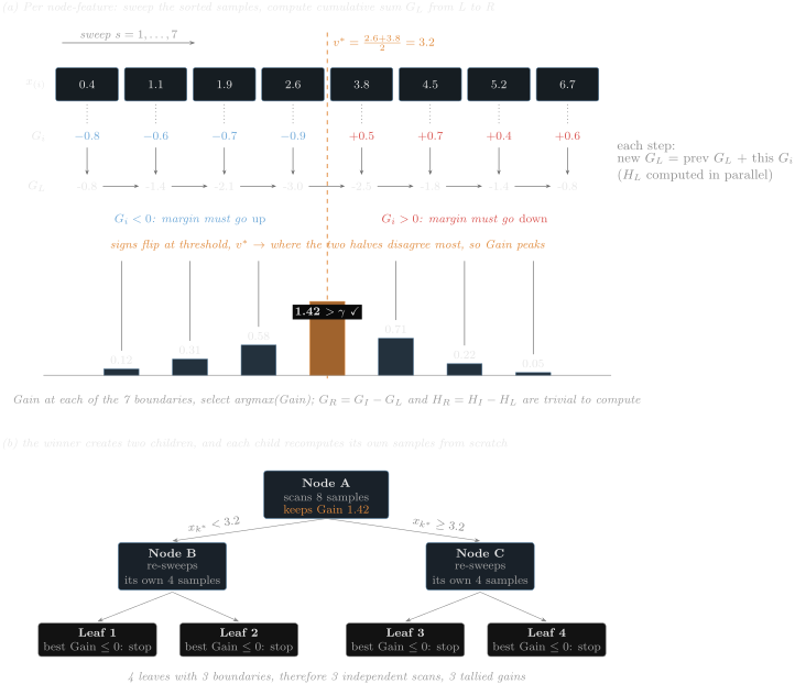
At a node with sample set I, for each feature k∈{1,…,d}:
- Take I in ascending (by convention) order of xik (pre-sorted once, globally; the node only walks its own subset): x(1),k≤x(2),k≤⋯≤x(∣I∣),k.
- Precompute totals GI=∑i∈IGi, HI=∑i∈IHi.
- Initialise GL←0, HL←0.
- Then sweep the boundaries s=1,…,∣I∣−1 and assign: GL←GL+G(s), HL←HL+H(s), GR←GI−GL, HR←HI−HL.
- Compute Gain and greedily select over all features k at threshold v that passes the cutoff: (k∗,v∗)=argmaxk,vGain(k,v).
All this turns what could've been an O(∣I∣2) operation per feature per node if done naively (rescanning all ∣I∣ samples at each of the ∣I∣−1 boundaries), into an O(1) procedure per boundary, and an O(∣I∣) sweep per feature per node after a one-off O(nlogn) sort per feature - very nice! The above, in turn, enables / unlocks more downstream optimization goodies such as cache-aware gradient prefetching, distributed workflows and more.
There's a slight wrinkle however in my explanation above due to simplifications for clarity. [3]The exact sweep over every one of the ∣I∣−1 boundaries, as I described, is the greedy recipe of plain GBDT (and XGBoost's exact method); the modern default hist uses a related histogram binning. XGBoost also offers an approximation method called the weighted quantile sketch (used for distributed / out-of-core training) - a method leveraging smaller sample approximation of the full thing for faster computation. Formally, for feature k define the Hessian-weighted rank rk(z)=∑i:xik<zHi/∑iHi, then pick only a handful of candidate thresholds {vk,1,…,vk,l} such that adjacent candidates differ in rank by less than some ϵ, giving roughly 1/ϵ candidates to sweep instead of ∣I∣−1. Intuitively, the idea is to build a histogram "sketch" with bins that hold equal amounts of uncertainty (H) instead of counts, and only test the bin edges, which is a much smaller set to sweep over!
Inbuilt Handling of Missing Values
Last but not least of the things to highlight, XGBoost has an inbuilt mechanism to deal with missing values in an effective way (super helpful in almost all real world datasets where data is never completely observable). In short, at each node, it checks which branch is best to put the missing value data points to (L or R), and directly dumps all the missing value points to the side that maximizes the Gain.
Gain∗=max(Gain(IL∪Imissing,IR),Gain(IL,IR∪Imissing))This is obvious in hindsight and almost too simple to believe, but it turns out to be very effective in practice, making XGBoost super accommodating to sloppy datasets.
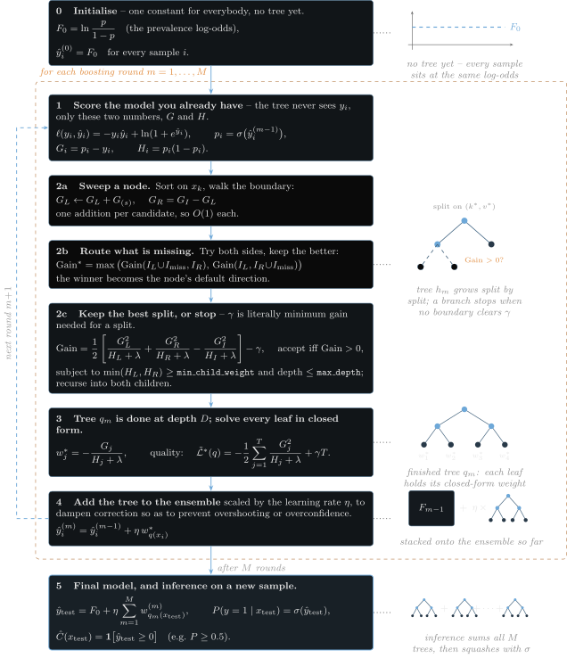
Okay, the above is a lot to take in, and indeed deserves a more thorough treatment to fully illustrate its depth and profoundness. However, I'll stop here and leave it as further reading, or perhaps a fuller in-depth essay if there's a demand for it. Fig 5 provides an overview of what we've discussed here to summarize things.
Why Does it Work so Well?
After all that exposition, we now turn our attention to the question oft-asked "why is XGBoost so good?". Indeed, there've been multiple times with which I've been forwarded this question and other similar ones along the lines of "why is X (e.g. neural net) not better than XGBoost [in tabular tasks]"?
The answer is context-dependent as one would expect. Note that we're only discussing in the context of tabular datasets and tasks here, which is where XGBoost is most applied - there's little doubt that outside of this domain, Deep Neural models are the reigning champions. Now back to the question at hand - in order to focus the argument, let's narrow our discussion to XGBoost (GBDT) vs Deep Neural Networks (DNN) such as Transformer and Deep Tabular Network.
First, for the positives of DNN. In terms of expressivity, DNN are definitely much more powerful in this regard than XGBoost, so they can represent a far wider class of function mappings compactly (universal approximation, benefits of depth). Not only that, modern Deep Tabular Networks like TabPFN have shown remarkable abilities with in-context learning that's very sample efficient yet performant, being able to learn with just hundreds to thousands of samples. At its limit, even zero-shot transfers without any task-specific training data at all for certain domains; of course, this excludes the pre-training of the transformer on a general corpus. This could be very useful indeed for tasks with very little available data or labels in cold-start settings, or for quick ad hoc tasks where one needs to make a prediction on a specific context without first training a model - hence, I'm very excited to see where this will go!
That being said, in a majority of real-world tasks, we do have a lot of available data - think of any products such as Stripe or Instagram, and at their scale, data abundance is definitely not a problem. Plus, DNN are very compute heavy, being slow to train and serve unlike XGBoost which is super snappy, sufficient to meet the high SLA / TPS requirements of real-time systems without needing a GPU; great news for those with a heavy compute backlog! On the other side of the train-serve equation, non-neural models like XGBoost are also endowed with very quick training speed, paired with the ability to ingest huge datasets (>100M rows) via lazy streaming, thereby making it much faster to iterate with unlike the lumbering DNN.
Now, other than the obvious and logistical (compute) reasons, XGBoost also admits certain very helpful properties in its learning process as well! The flipside problem with DNN on their expressivity is the issue of overfitting, which comes at no surprise to any practitioners - it's not easy to "tame" a DNN so it wouldn't just memorize the dataset trivially. XGBoost on the other hand, is capable of dealing with the issue of overfitting naturally - as we've seen previously, all GBDT like XGBoost does, is learn how to partition the feature space into axis-aligned "rectangles" to segment the samples cleanly.
It is precisely the "constraint" of only being able to learn additive axis-aligned rectangular partitions - no rotations or bending! - that naturally induces a structural regularization, thereby preventing it from overfitting easily, e.g. it cannot learn arbitrarily smooth feature segmentation boundaries. Added to that, the margin maximizing effect of boosting in the small-η limit further forces an additional constraint in a useful way, preventing degeneration into trivial margin-agnostic segmentation that's highly irregular or jagged. In short, the structure of the trees themselves with their margin maximizing tendency provides built-in, implicit regularization mechanics to XGBoost, on top of other explicit regularizing forces such as γ, λ and co!
Upon some consideration, one could also notice certain congruency between tabular datasets and the structure of XGBoost we just covered in prior sections. For example, the feature manifold of tabular data is typically irregular (e.g. non-smooth with sharp thresholds) such as credit scores - which have categorical spans, where a certain score-band means "poor" while being above a certain score indicates an "excellent" credit risk profile - or glucose level - above certain values, we classify as excessive; hyperglycemia or hypoglycemia - and so on. DNN are biased towards smooth, low frequency boundaries, whereas GBDT like XGBoost's staircase-like boundaries match this inductive bias perfectly. Also, in tabular data, columns are oftentimes "self-describing" or individually-meaningful - annual income and age are by themselves salient and are widely used "abstractions" - which the axis-aligned nature of GBDT naturally assumes for free without needing to manually "impose" any additional constraints.
For example, take the income and age columns of a dataset, and replace them with their sum or differences. No information has been lost, it's just written along a rotated pair of axes, which may or may not be a useful joint feature for the task at hand; worse if it's destructive! Tabular data arrives already with a natural basis imposed by whoever created the columns, so a learner that is invariant to rotation has to rediscover that orientation from scratch, mixing together features with very different statistical properties along the way, which may not yield any useful signal. GBDT on the other hand, naturally leans into these given tabular priors nicely.
Last but not - exhaustively - least, is the ability of GBDT to easily and naturally ignore uninformative features, of which there usually are in any real world datasets, by simply not splitting on those features, and be able to do so for free as part of its Gain computation's factor already, unlike the DNN which could degrade due to relative influences; though, this is more of a problem of plain feedforward networks as newer Transformer-based models like FT-Transformer have accounted for with their per-feature tokenizer.
All these taken together, are reasons why Gradient Boosted Decision Trees like XGBoost normally rank so well in tabular or structured learning tasks and benchmarks, and are so often preferred by production teams even to this day - it's just a tabular-shaped solution to a tabular world, and it's zippy too!
| XGBoost (GBDT) | DNN (Transformer, Deep Tabular) | |
|---|---|---|
| Expressivity | Additive axis-aligned rectangle partitions - no rotations or bending | Much more powerful; represents a far wider class of function mappings compactly |
| Small data, cold start | Needs task-specific training data | In-context learning that is very sample efficient yet performant; at its limit even zero-shot for certain domains |
| Data abundance | The regime it is built for (the usual case) | Advantage narrows once data is abundant - at Stripe or Instagram scale, data is definitely not a problem |
| Compute and latency | Super snappy; CPU alone is sufficient to meet the high SLA / TPS requirements of large scale systems | Very compute heavy and slow; takes specialized optimization and GPUs to catch up |
| Training and iteration | Much faster to train, and therefore iterate rapidly | Lumbering by comparison |
| Overfitting | The constraint itself induces a structural regularization, plus the margin maximizing tendency and +λ - a built-in, implicit regularization | Not easy to "tame" so it wouldn't just memorize the dataset trivially |
| Tabular inductive bias | Matches irregular features with sharp thresholds (credit scores, glucose levels) perfectly | Biased towards smooth, low frequency segmentations |
| Independent columns | Columns are self-describing and individually meaningful; tabular data arrives with a natural basis that the axis-aligned nature leans into for free | A rotation-invariant learner has to rediscover that orientation from scratch, mixing features with very different statistical properties along the way |
| Uninformative columns | Ignored by simply not splitting on those features, essentially for free - as part of its Gain computation already | Could degrade due to relative influence (more of a problem of plain MLP; newer Transformer-based models like FT-Transformer have accounted for it with their per-feature tokenizer) |
Closing Words
Now dear Readers, we're at the end of our journey. That being said, I must point out a few areas of deficiencies and shortcuts I have taken in this exposition for clarity and brevity, lest I be stoned by the but-ackchyually-police!
First off, the enumeration of XGBoost's mechanics is incomplete and only covers core mechanics that I believe to be necessary and sufficient. For example, there's no mention of how the tree is grown to max_depth and then performs backward-pruning, the full treatment of the weighted quantile sketch and approximate split finding, how it handles categorical data, how it performs multicore training, how additional improvements have allowed it to stream and train lazily for datasets that won't fit in memory, how it computes feature importance, and many more. For those, I would direct the motivated reader to the original paper and the latest official documentation.
Furthermore, the theoretical treatment is also rather lackluster as it's not intended to be a textbook. However, there's a great deal to be gleaned from and pondered on via a more rigorous treatment in depth. For example, how the learning procedure can be seen as an ℓ1 walk on the axis-aligned path in the function space, how margin theory can help us understand why it can learn so well, what are its convergence properties and levers that affect it most directly, which in turn help us build intuition to understand why a turn-up-the-rounds-to-11-and-lower-the-learning-rate is a decent strategy in general when tuning XGBoost.
Last and most importantly in my opinion, is the omission on how the model behaves in extreme settings such as dealing with a dataset with huge prevalence imbalance - which is very common in domains such as credit-card fraud, cancer diagnosis, and many others - and as a result this impacts calibration and uncertainty quantification, which in turn affects downstream dependencies such as the policy engine and so on. Other just as important considerations are on dealing with a drifting non-stationary environment, and when uncertainty estimation is unreliable or otherwise. Perhaps these can be addressed in a future write-up on operational considerations in practice.
That's the tour, and I hope that this has been helpful and not too dreadful of a read. For any inquiries, errors and corrections, or simply a conversation on the topic, feel free to reach out and I shall make the best endeavor to reply swiftly. Ta-ta!
References
- [1]Benchmarking state-of-the-art classification algorithms for credit scoring: An update of researchEuropean Journal of Operational Research. [Online]. Available: https://doi.org/10.1016/j.ejor.2015.05.030
- [2]A data-driven approach to predict the success of bank telemarketingDecision Support Systems. [Online]. Available: https://doi.org/10.1016/j.dss.2014.03.001
- [3]Explainable machine-learning predictions for the prevention of hypoxaemia during surgery - Nature Biomedical EngineeringNature. [Online]. Available: https://doi.org/10.1038/s41551-018-0304-0
- [4]M5 accuracy competition: Results, findings, and conclusionsInternational Journal of Forecasting. [Online]. Available: https://doi.org/10.1016/j.ijforecast.2021.11.013
- [5]XGBoost: A Scalable Tree Boosting SystemarXiv.org. [Online]. Available: https://arxiv.org/abs/1603.02754
- [6]The ASHRAE Great Energy Predictor III competition: Overview and resultsarXiv.org. [Online]. Available: https://arxiv.org/abs/2007.06933
- [7]TabArena: A Living Benchmark for Machine Learning on Tabular DataarXiv.org. [Online]. Available: https://arxiv.org/abs/2506.16791
- [8]Higgs Boson Discovery with Boosted TreesPMLR. [Online]. Available: https://proceedings.mlr.press/v42/chen14.html
- [9]Deep Learning for Credit Scoring: Do or Don't?European Journal of Operational Research. [Online]. Available: https://doi.org/10.1016/j.ejor.2021.03.006
- [10]Performance of CatBoost and XGBoost in Medicare Fraud DetectionIEEE ICMLA. [Online]. Available: https://doi.org/10.1109/ICMLA51294.2020.00095
- [11]Why do tree-based models still outperform deep learning on tabular data?arXiv.org. [Online]. Available: https://arxiv.org/abs/2207.08815
- [12]Tabular Data: Deep Learning is Not All You NeedarXiv.org. [Online]. Available: https://arxiv.org/abs/2106.03253
- [13]When Do Neural Nets Outperform Boosted Trees on Tabular Data?arXiv.org. [Online]. Available: https://arxiv.org/abs/2305.02997
- [14]Accurate predictions on small data with a tabular foundation model | Naturenature.com. [Online]. Available: https://www.nature.com/articles/s41586-024-08328-6
- [15]A Closer Look at TabPFN v2: Understanding Its Strengths and Extending Its CapabilitiesarXiv.org. [Online]. Available: https://arxiv.org/abs/2502.17361
- [16]Classification and Regression TreesTaylor & Francis. [Online]. Available: https://doi.org/10.1201/9781315139470
- [17]Elements of Statistical Learning: data mining, inference, and prediction. 2nd Edition.hastie.su.domains. [Online]. Available: https://hastie.su.domains/ElemStatLearn/
- [18]Boosting: Foundations and AlgorithmsMIT Press. [Online]. Available: https://mitpress.mit.edu/9780262526036/boosting/
- [19]Cryptographic Limitations on Learning Boolean Formulae and Finite AutomataJournal of the ACM. [Online]. Available: https://doi.org/10.1145/174644.174647
- [20]The Strength of Weak LearnabilityMachine Learning (Springer). [Online]. Available: https://doi.org/10.1007/BF00116037
- [21]A Decision-Theoretic Generalization of On-Line Learning and an Application to BoostingJournal of Computer and System Sciences. [Online]. Available: https://doi.org/10.1006/jcss.1997.1504
- [22]Boosting the Margin: A New Explanation for the Effectiveness of Voting MethodsThe Annals of Statistics. [Online]. Available: https://doi.org/10.1214/aos/1024691352
- [23]Greedy Function Approximation: A Gradient Boosting MachineThe Annals of Statistics. [Online]. Available: https://doi.org/10.1214/aos/1013203451
- [24]Additive Logistic Regression: A Statistical View of BoostingThe Annals of Statistics. [Online]. Available: https://doi.org/10.1214/aos/1016218223
- [25]Approximation by superpositions of a sigmoidal functionMathematics of Control, Signals, and Systems. [Online]. Available: https://doi.org/10.1007/BF02551274
- [26]Benefits of Depth in Neural NetworksPMLR. [Online]. Available: https://proceedings.mlr.press/v49/telgarsky16.html
- [27]TabPFN: A Transformer That Solves Small Tabular Classification Problems in a SecondarXiv.org. [Online]. Available: https://arxiv.org/abs/2207.01848
- [28]TabLLM: Few-shot Classification of Tabular Data with Large Language ModelsarXiv.org. [Online]. Available: https://arxiv.org/abs/2210.10723
- [29]Using XGBoost External Memory Version — xgboost 3.4.1 documentationxgboost.readthedocs.io. [Online]. Available: https://xgboost.readthedocs.io/en/stable/tutorials/external_memory.html
- [30]Feature Selection, L1 vs. L2 Regularization, and Rotational InvarianceICML 2004. [Online]. Available: https://doi.org/10.1145/1015330.1015435
- [31]Boosting as a Regularized Path to a Maximum Margin ClassifierJournal of Machine Learning Research. [Online]. Available: https://jmlr.org/papers/v5/rosset04a.html
- [32]On the Spectral Bias of Neural NetworksPMLR. [Online]. Available: https://proceedings.mlr.press/v97/rahaman19a.html
- [33]Revisiting Deep Learning Models for Tabular DataarXiv.org. [Online]. Available: https://arxiv.org/abs/2106.11959